PowerBI SmartPivot 101: all you need to get started

Joel Monteiro
May 8, 2019PowerBI SmartPivot 101 is the complete guide for our first product for 2019. Much like the rest of our PowerBI Tiles family, PowerBI SmartPivot was born to answer our clients’ problems. From there, it was adjusted and spun into a ready to market product. In this case, we had clients in the retail sector that extensively used Excel PivotTables in their daily activity. Their woes included a high dependency on IT staff to connect databases to Excel, the lack of granularity provided by Excel alone, and, perhaps most importantly, the time it took to filter their PivotTables when analyzing a wide range of items, a common occurrence in retail.
Unlike other members of its family, namely PowerBI Tiles Pro and PowerBI Robots, you don’t need to be a Power BI user to take full advantage of PowerBI SmartPivot. However, the ability to connect Excel to Power BI is unique to PowerBI SmartPivot and one of its main features.
Follow this PowerBI SmartPivot 101 to learn how to use its main functions:
1. What is PowerBI SmartPivot and who is it for?
PowerBI SmartPivot is an Excel add-in aimed at professionals who regularly work with PivotTables. PowerBI SmartPivot introduces several features that make their life easier. These include the ability to connect OLAP data cubes and Power BI to Excel, scan all data in an analytical model, apply filters in bulk instead of individually ticking a PivotTable’s checkboxes and create granular table reports with ease.
2. Downloading and installing PowerBI SmartPivot
You can try PowerBI SmartPivot for free by downloading a full-featured 30-day trial version. If you enjoy it, an annual license is available for 99.99€. We also provide discounts for organizations that wish to purchase multiple licenses.
After downloading PowerBI SmartPivot, extract the file and double click it to run the installation wizard. Follow the steps and click finish. Open Excel and you should see a grayed-out SMARTPIVOT tab.
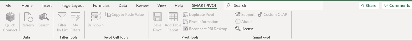
Click the License button and introduce the key emailed to the address you used to register for the PowerBI SmartPivot trial. Once validated, all options will become available.

NOTE: if you don’t see the SMARTPIVOT tab in Excel, go to File > Options and click the Add-ins tab.
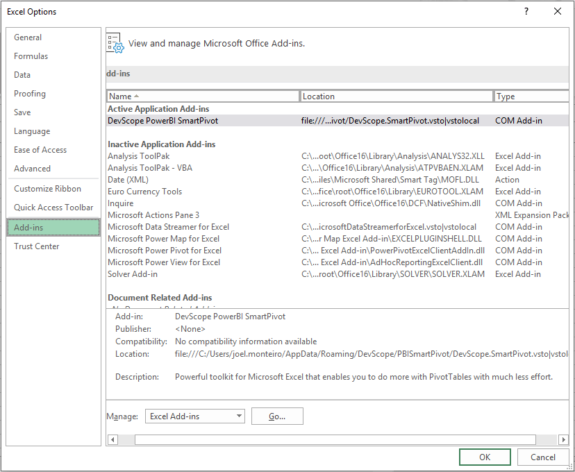
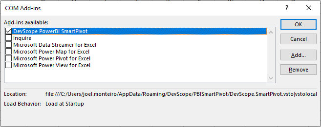
From the Manage dropdown menu, select COM Add-ins and click the Go button. Make sure the DevScope PowerBI SmarPivot check-box is ticked and click OK.
The SMARTPIVOT tab should now be visible. If you still can’t see it, please email our support team.
3. Connecting OLAP cubes and Power BI to Excel
In order to connect a Power BI dataset to Excel, you must first open it in Power BI Desktop. Once you do, go to the SMARTPIVOT tab in Excel and click QuickConnect. You should see it in the list of connections available.
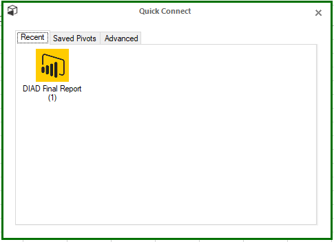
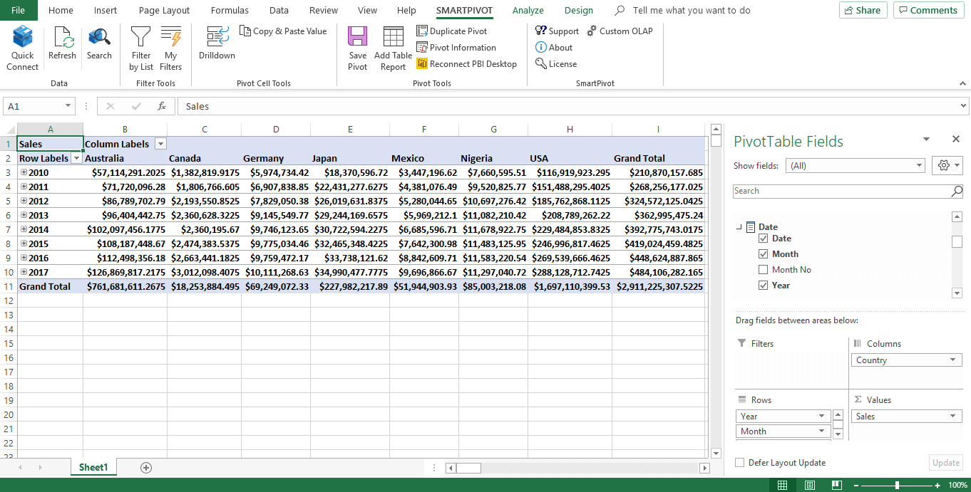
Double-click it and confirm the range. The PivotTable Fields will appear in the panel on the right. Select which fields you want to add to your PivotTable or drag them to the preset areas below.
4. Using the search function
PowerBI SmartPivot’s search function greatly expands on what Excel can do by itself, allowing users to find exactly what they’re looking for, regardless of the complexity of their analytical model.
To use it, select any cell in your PivotTable and click the search icon in the menu. A new pane will open next to the PivotTable Fields selection.
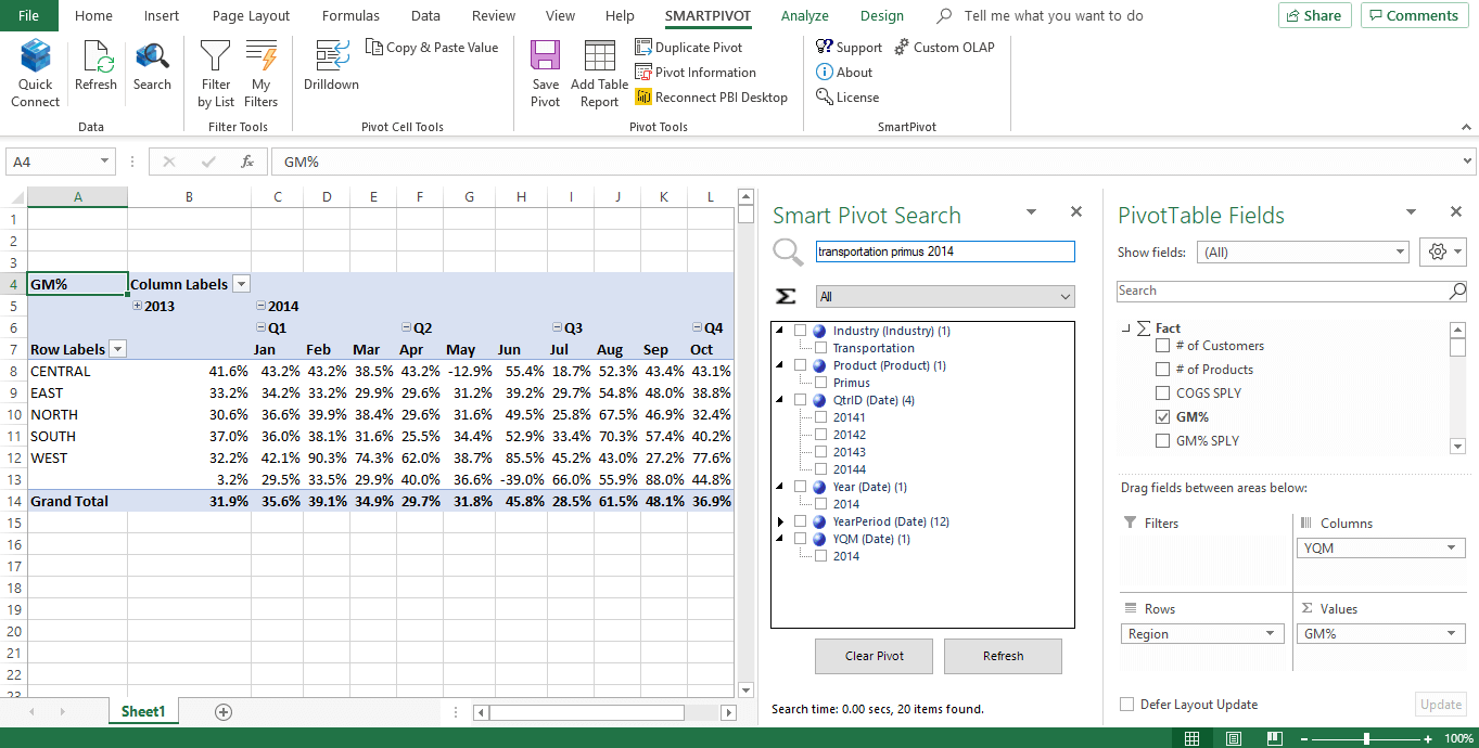
You can place any queries in the search field to find exactly the data you’re looking for. In the example below, we’ll ask PowerBI SmartPivot for the gross margin percentage (GM%) of transportation of Primus in 2014. PowerBI SmartPivot will instantly scan your data model and present you with a list of the fields that best match your query.
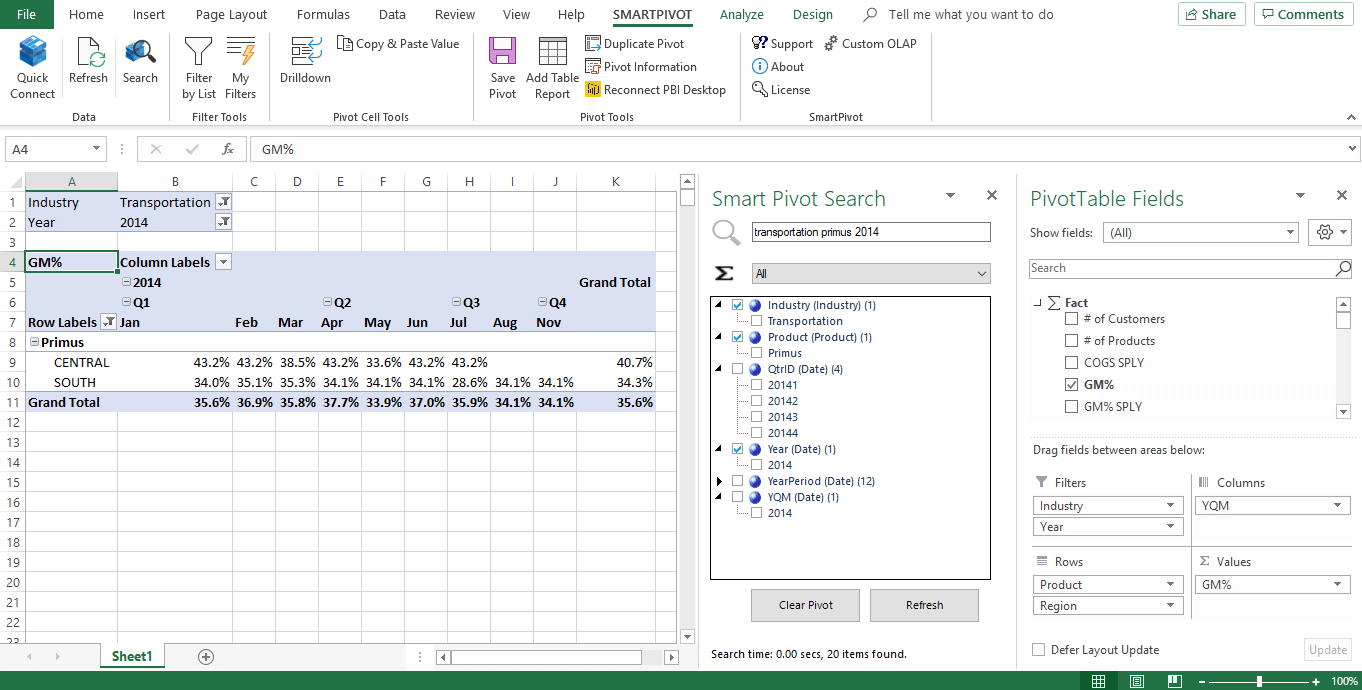
Check the boxes from the list to add that data to a new PivotTable.
5. Filtering a PivotTable by a list of values
The more data you have in an analytical model, the harder it is to find what you want. Even when you know where to look, it may take some time picking the values for your PivotTable since Excel only allows you to select or deselect all values at the same time.
This may not be a problem when working with a small PivotTable, but becomes a major annoyance when you’re working with hundreds or thousands of values you have to individually pick. This became apparent when working with our retail clients. Their PivotTables often have hundreds or thousands of products, which means spending several minutes checking boxes. Earlier last year, we launched Filter by List for Power BI on Microsoft’s AppSource for free. It’s now integrated into Excel as one of the tools in PowerBI SmartPivot.
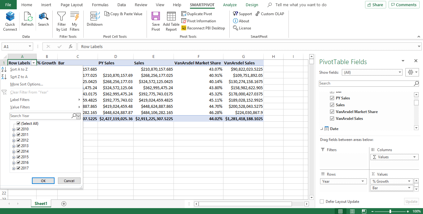
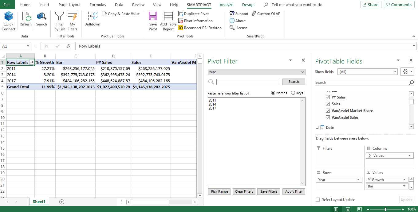
Using it couldn’t be simpler. With at least a cell of your PivotTable selected, click the Filter by List icon from the menu to open the Pivot Filter pane. Write or paste the list of values you wish to filter your list by and click Apply Filter.
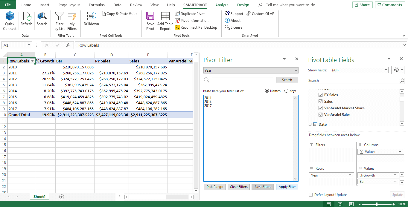
Your PivotTable will change and reflect those values.
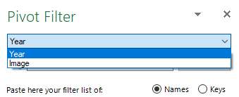
NOTE: If your PivotTable has more than one hierarchy, make sure you select the correct one from the dropdown list.
If you plan on using the same filter recurrently, it’s a good idea to save it – just hit the Save Filter button after applying it. PowerBI SmartPivot will save the values in your filter and direct you to a page where you can apply, update, or delete previously saved filters.
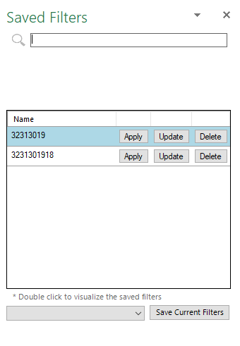
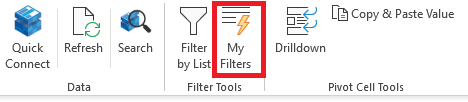
To access your saved filters, select any cell on the PivotTable and click the My Filters button from the menu. This will open a pane with your list of saved filters.
6. Creating a granular table from an OLAP cube
Lastly, we’ll cover the ability to quickly create a granular table report by selecting its fields from a list. To do it, select a cell containing one of the results in your PivotTable and click Add Table Report from the menu. A window containing all possible fields will open.
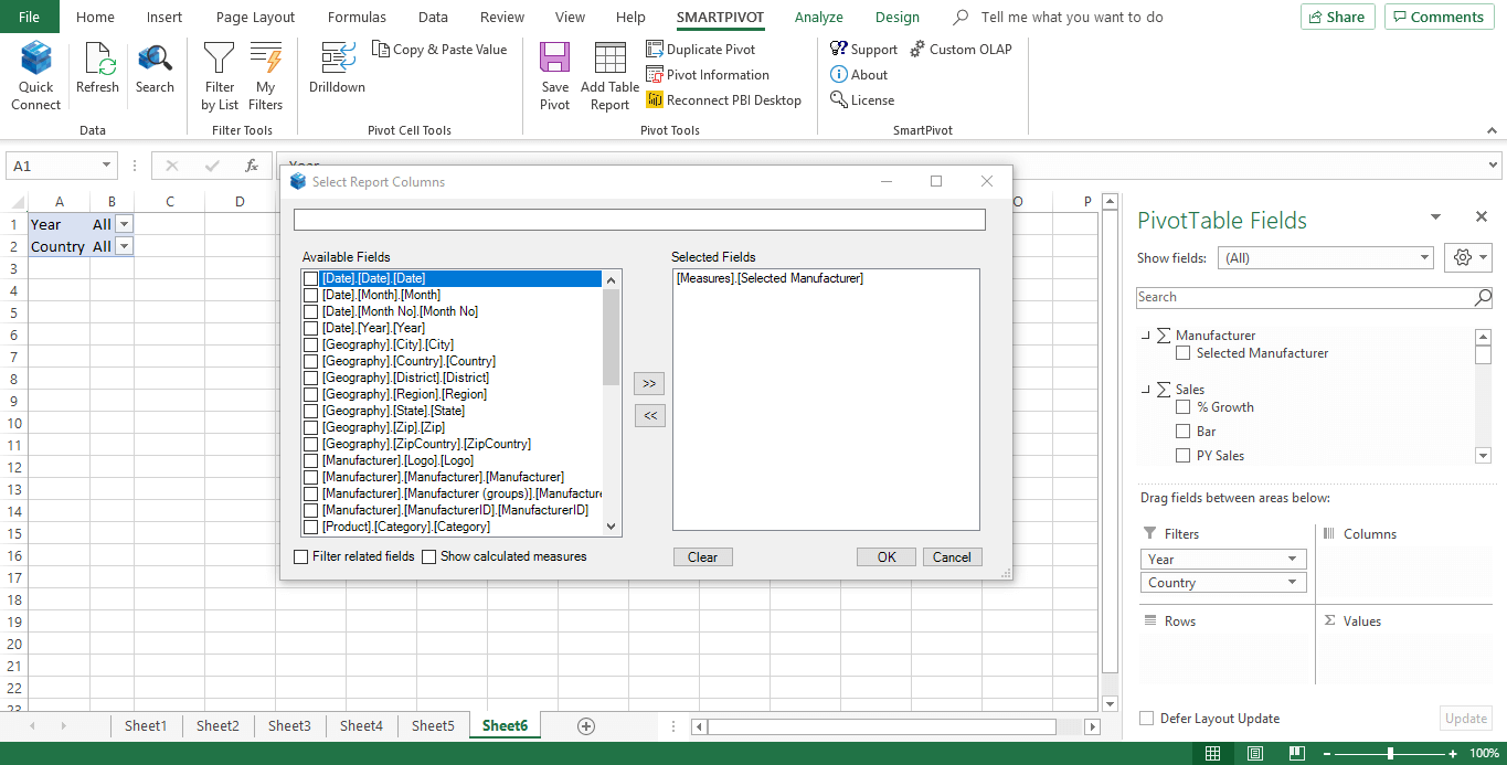
To create a table, pick a field from the Available Fields and add it to the Selected Fields section.
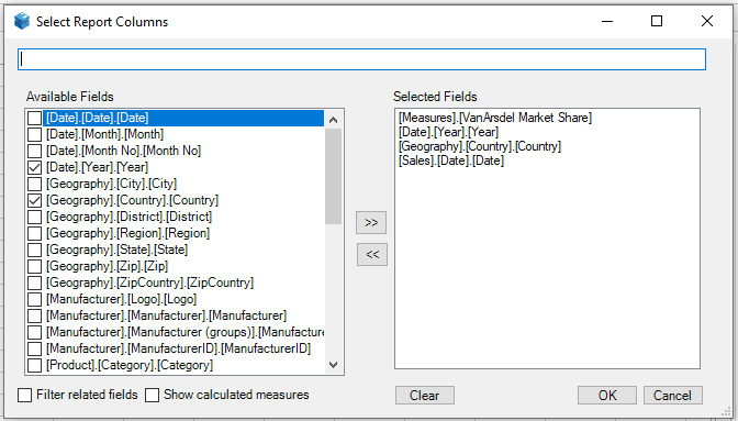
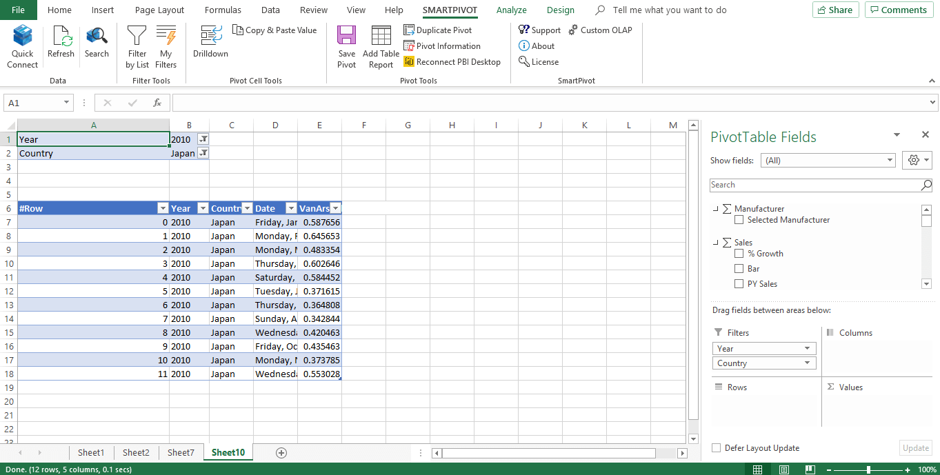
When you’re done, click ok to create your table instantly in a new Excel sheet.
If you still have any questions regarding PowerBI SmartPivot, please check the product’s FAQs or contact us by email.
Thank you for reading this PowerBI SmartPivot 101. There are other features we didn’t cover in this PowerBI SmartPivot 101 because we feel are self-explanatory. Nevertheless, if you need any help using them, let us know in the comments or contact our team.

Introducing PowerBI SmartPivot. Try it today for free!
We’re proud to announce PowerBI SmartPivot, a Microsoft Excel add-in that introduces several new features aimed at boosting the productivity of advanced [...]